计算机视觉上机实践一图像的基本操作

一、实验目的

通过本次实验，掌握图像的读取、显示、保存、绘制等基本操作；

熟悉图像的灰度直方图原理，并对图像进行灰度变换和颜色空间变换；

能绘制自定义图像。

二、实验环境

硬件环境：一台笔电
软件环境：Windows10环境、Jupyter Notebook软件;

三、实验内容及代码实现

1. 读取、显示、保存图像

源文件lena.png:

# 1.读取、显示、保存Lena图像；(使用matplotlib库)

import numpy as np
import matplotlib.pyplot as plt
import matplotlib.image as mpimg 

# mipimg读取图片
lena = mpimg.imread('lean.png') 

plt.imshow(lena) # plt.imshow()函数负责对图像进行处理，并显示其格式
plt.axis('off') # 不显示坐标轴
plt.title('Lena.png') # 显示标题

# 保存图片
#bbox_inches='tight'表示指定将图表多余的空白区域裁减掉
plt.savefig('lean-new.png', bbox_inches='tight')  # 注意：保存需要在显示的前面，否则保存的图片会是空白

# 显示经imshow处理的图片
plt.show()

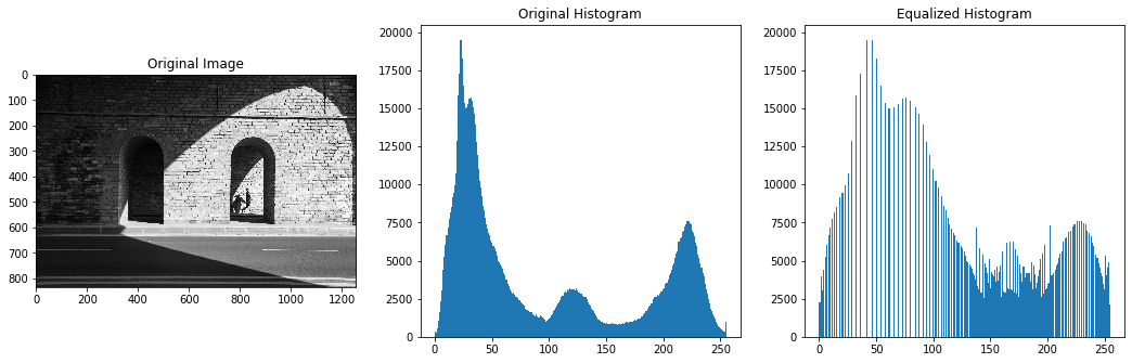
2.直方图均衡化

内容：选择一张有明暗对比的图片(网上找一张即可)，读取并绘制图像的直方图；对输入图像进行直方图均衡化并输出结果；

（1）使用Matplotlib库实现

# 2.选择一张有明暗对比的图片，读取并绘制图像的直方图；对输入图像进行直方图均衡化并输出结果；（使用Matplotlib库实现）

import numpy as np
import matplotlib.pyplot as plt
import cv2 # opencv读取的图片数值为BGR格式

# 读取并显示原始图像
original = cv2.imread('test.jpg') # 第2个参数flags表示标记位，读入灰度图片可用0作为实参替代
# 创建1个图形figure
plt.figure(figsize=(18, 18)) 
image1 = plt.subplot(3, 3, 1) # 为方便观察结果，这里创建了多个子图subplot
image1.set_title('Original Image')
plt.imshow(original)

# 原图的直方图
img = cv2.imread('test.jpg',0) # 第2个参数flags表示标记位，读入灰度图片可用0作为实参替代
# 这里使用Matplotlib库自带的计算并绘制直方图功能
image2 = plt.subplot(3, 3, 2)
image2.set_title('Original Histogram')
plt.hist(img.ravel(),256,[0,255]) # 绘制原图像的灰度直方图

# 均衡化后的直方图
img2 = cv2.equalizeHist(img)
image4 = plt.subplot(3, 3, 3)
image4.set_title('Equalized Histogram')
plt.hist(img2.ravel(),256,[0,255])
plt.show()

（2）使用opencv库实现

# 2.更好的阅读体验，使用subplot创建单个子图（使用opencv库实现）

import numpy as np
import matplotlib.pyplot as plt
import cv2

img = cv2.imread('test.jpg', 0) # 读取原始图的灰度度
img_eq = cv2.equalizeHist(img) # 用opencv库实现图像直方图均衡化

# opencv库calcHist()来计算直方图
hist = cv2.calcHist([img], [0], None, [256], [0,255]) # 第1个参数表示要计算的原图 
hist_eq = cv2.calcHist([img_eq], [0], None, [256], [0,255])

# 创建1个图形figure
plt.figure(figsize=(13, 13)) 
image1 = plt.subplot(2, 2, 1)
image1.set_title('Oringinal Image')
plt.imshow(img, cmap='gray') # cmap:颜色图谱（colormap),这里是绘制灰图

# 均衡化后的图片
image2 = plt.subplot(2, 2, 2)
image2.set_title('Equalized Image')
plt.imshow(img_eq,cmap='gray')

# 原图的直方图
image3 = plt.subplot(2, 2, 3)
image3.set_title('Oringinal Histogram')
plt.plot(hist)

# 均衡化后的直方图
image4 = plt.subplot(2, 2, 4)
image4.set_title('Equalized Histogram')
plt.plot(hist_eq)

plt.show()

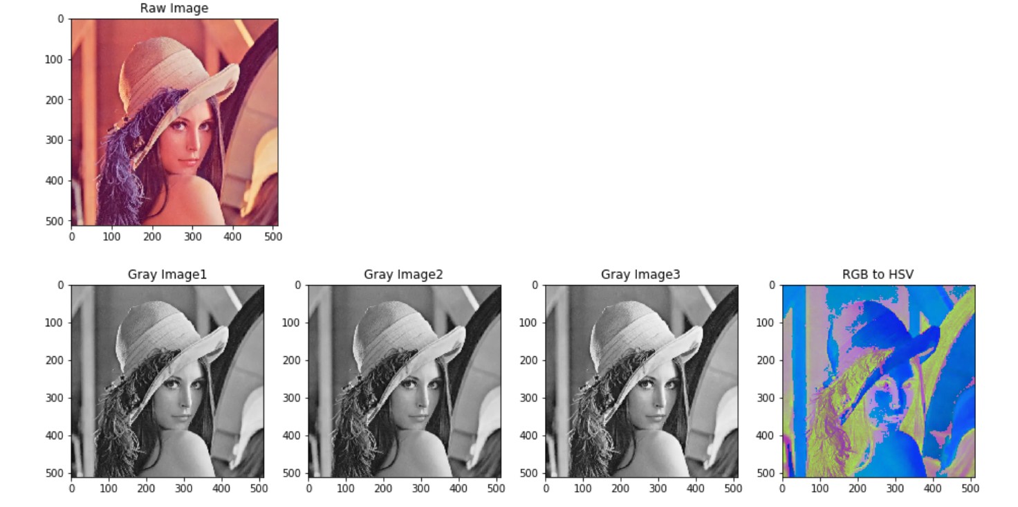
3. 对图像进行灰度变换、颜色空间转换等基本操作

# 3.对读入图像进行灰度变换、颜色空间转换等基本操作；

import numpy as np
import matplotlib.pyplot as plt
import cv2

# 读取图像,opencv读取图像是BGR顺序
img = cv2.imread('lean.png') 

# 正确显示图片
plt.figure(figsize=(8, 8)) 
image1 = plt.subplot(1, 2, 1)
image1.set_title('Raw Image')
plt.imshow(cv2.cvtColor(img.astype(np.uint8), cv2.COLOR_BGR2RGB)) # 保证显示出的图像是RGB顺序

# 进行灰度变换：RGB to GRAY
# 方法1，使用公式：Gray = 0.2989*R+0.5870*G+0.1140*B
img1 = 0.2989 * img[:,:,2] + 0.5870 * img[:,:,1] + 0.1140 * img[:,:,0] # 分别取出img数组中的RGB二维数组计算
plt.figure(figsize = (16, 16))
image2 = plt.subplot(4, 4, 1)
image2.set_title('Gray Image1')
plt.imshow(img1, cmap='gray')

# 方法2，使用openCV自带函数进行转换
image3 = plt.subplot(4, 4, 2)
image3.set_title('Gray Image2')
plt.imshow(cv2.cvtColor(img.astype(np.uint8), cv2.COLOR_BGR2GRAY), cmap='gray')

# 方法3，根据Gray公式自定义函数将RGB转为灰度图（类似方法一）
def rgb2gray(rgb):
    return np.dot(rgb[:, :,:3], [0.299, 0.587, 0.114]) # 进行向量点乘
gray = rgb2gray(img)
image4 = plt.subplot(4, 4, 3)
image4.set_title('Gray Image3')
plt.imshow(gray, cmap='Greys_r')

# 颜色空间转换, RGB to HSV
img2 = cv2.cvtColor(img, cv2.COLOR_BGR2HSV) # HSV常用于分割指定颜色的物体
image5 = plt.subplot(4, 4, 4)
image5.set_title('RGB to HSV')
plt.imshow(img2)

plt.show()

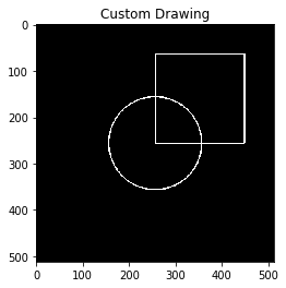
4. 自定义图像绘制

内容：定义一个像素为512*512的图像平面，黑色背景，在该图像上面生成一个正方形和圆，要求正方形的四个点为A（256，64）、B（256，256）、C（448，256）、D（448，64）；要求圆的半径r=100，圆心为（256，256）。

# 4.自定义图像绘制。定义一个像素为512*512的图像平面，黑色背景，在该图像上面生成一个正方形和圆，
#   要求正方形的四个点为A（256，64）、B（256，256）、C（448，256）、D（448，64）；
#   要求圆的半径r=100，圆心为（256，256）。

import numpy as np
import matplotlib.pyplot as plt

# 创建一个像素为512*512的图像平面，黑色背景
img = np.zeros((512, 512, 3), dtype=np.uint8)

# 定义正方形的四个点
A = (256, 64)
B = (256, 256)
C = (448, 256)
D = (448, 64)

# 绘制正方形
cv2.line(img, A, B, (255, 255, 255), 2)  # AB
cv2.line(img, B, C, (255, 255, 255), 2)  # BC
cv2.line(img, C, D, (255, 255, 255), 2)  # CD
cv2.line(img, D, A, (255, 255, 255), 2)  # DA

# 定义圆心和半径
center = (256, 256)
r = 100

# 绘制圆
cv2.circle(img, center, r, (255, 255, 255), 2)

# 显示图像
plt.imshow(img)
plt.title('Custom Drawing')
plt.show()