数据挖掘与机器学习 线性回归设计 实训1
数据挖掘与机器学习 线性回归设计 实训1
(1)实训目的
1.掌握回归的基本思想;
2.掌握梯度法的基本原理 。
(2)主要内容
1.实现一元线性回归;
2.画出散点图、回归参数与迭代次数的变化曲线;
3.分析不同数据变化对回归结果的影响。
(3)具体处理步骤
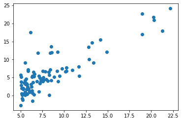
1. 导入数据集,绘制数据的散点图
1 | import numpy as np |
1 | data.shape # 原数据集形状,n行m列 |
(97, 2)
2. 对特征进行归一化处理
1 | def featureNormalize(x): # (特征值x的取值差别较大)需消除特征值的量纲 |
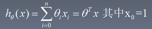
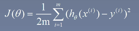
3.1 定义损失函数 h_theta是预测函数(假设函数),j_theta是损失函数
1 | def computeCost(x, y, theta): # 损失函数j_theta |
3.2 梯度下降算法
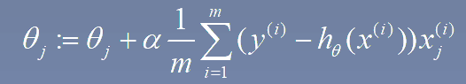
利用公式 theta : 是预测函数每项的系数,times:梯度下降次数,alpha:梯度下降参数变化率
1 | def gradientDescent(x, y, theta, times, alpha): |
4. 计算求得的直线
1 | x_orgin=x # 分别取x,y这列的值 |

1 | print('预测函数: y = %f + %f * x' % (theta[0], theta[1])) |
预测函数: y = 5.825092 + 5.884855 * x
x=3, y = 23.479657
5. 画损失函数,损失随迭代次数变化的曲线
1 | x_times = np.linspace(1,times,times) |
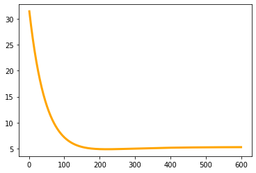
6. 结果分析
分析可知,当迭代次数到200次左右时,损失函数趋于收敛损失值达到最小值,迭代次数太多,可能使得出现过拟合现象
alpha 越小时,即步长越小,使得训练过程中的变化速度较慢,但可能更易于损失函数收敛
(4)参考资料
本博客所有文章除特别声明外,均采用 CC BY-NC-SA 4.0 许可协议。转载请注明来自 AriesfunのBlog!
相关推荐


评论