数据分析与可视化 上机实践1(Numpy 数值计算)
一、实践目的
1.掌握 Numpy 库的使用方法。
2.灵活应用 Numpy 库解决数值计算和图像处理的相关问题。
二、彩色向灰度图转换原理
图像是由若干个像素组成,每个像素有明确的位置和被分配的颜色值。
一张图像就构成了一个像素矩阵。彩色图像的每个像素由 R、G、B 分量构成;分量值介于 0到255 之间。灰度图像是每个像素只有一个采样颜色的图像,显示为从最 暗黑色到最亮的白色的灰度,取值范围 0到255。
彩色图像向灰度图像转换的常用公式为:
Gray = R * 0.299 + G * 0.587 + B * 0.114
利用矩阵运算,即可将彩色图像转换为灰度图像。
三、实践内容要求
数组的创建
(1)创建全 0 数组,全 1 数组,随机数数组;
(2)创建一个数值范围为 0~1,间隔为 0.01 的数组。
任意创建一个二维数组,对其维度进行操作
(1)将数组的行变列;
(2)返回最后一个元素;
(3)返回第 2 到第 4 个元素;
(4)返回逆序数组。
任意创建两个二维的数组 arr1、arr2,对两个数组进行四则运算:arr1+arr2、 arr1-arr2、arr1*arr2、arr1/arr2。
创建数组 arr3=[3 6 9 3 1 5 7 2],分别完成排序、去重、总和、累计和、均 值、标准差、方差、最小值和最大值的统计。
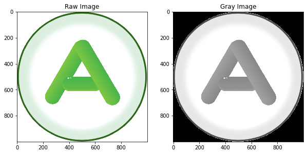
了解图像的构成,结合 Matplotlib 和 NumPy 实现彩色图像到灰色图像的 转换,将彩色图像转换为灰度图像。
5 的实验步骤包括以下几个: 1. 导入 numpy 和 matplotlib 模块; 2. 读取彩色图像(plt.imread); 3. 显示彩色图像(plt.imshow); 4. 通过数组间的运算,计算灰度图像的像素值; 5. 显示灰度图像
四、完成情况
1
2
3
4
5
6
7
8
9
10
11
12
13
14
15
|
import numpy as np
a = np.zeros((3, 3))
print(a)
b = np.ones((3, 3))
print(b)
c = np.random.random((3, 3))
print(c)
a = np.arange(0, 1, 0.01)
print(a)
|
1
2
3
4
5
6
7
8
9
10
11
12
13
14
15
16
17
| [[0. 0. 0.]
[0. 0. 0.]
[0. 0. 0.]]
[[1. 1. 1.]
[1. 1. 1.]
[1. 1. 1.]]
[[0.59795796 0.47702449 0.90950593]
[0.27112045 0.53074871 0.70262116]
[0.97665706 0.43174363 0.17952276]]
[0. 0.01 0.02 0.03 0.04 0.05 0.06 0.07 0.08 0.09 0.1 0.11 0.12 0.13
0.14 0.15 0.16 0.17 0.18 0.19 0.2 0.21 0.22 0.23 0.24 0.25 0.26 0.27
0.28 0.29 0.3 0.31 0.32 0.33 0.34 0.35 0.36 0.37 0.38 0.39 0.4 0.41
0.42 0.43 0.44 0.45 0.46 0.47 0.48 0.49 0.5 0.51 0.52 0.53 0.54 0.55
0.56 0.57 0.58 0.59 0.6 0.61 0.62 0.63 0.64 0.65 0.66 0.67 0.68 0.69
0.7 0.71 0.72 0.73 0.74 0.75 0.76 0.77 0.78 0.79 0.8 0.81 0.82 0.83
0.84 0.85 0.86 0.87 0.88 0.89 0.9 0.91 0.92 0.93 0.94 0.95 0.96 0.97
0.98 0.99]
|
1
2
3
4
5
6
7
8
9
10
11
12
13
|
import numpy as np
a = np.arange(9).reshape(3, 3)
print(a)
print(a.T)
print(a[2, 2])
print(a[0, 2])
print(a[1, : 2])
print(a[: : -1, : : -1])
|
1
2
3
4
5
6
7
8
9
10
11
12
| [[0 1 2]
[3 4 5]
[6 7 8]]
[[0 3 6]
[1 4 7]
[2 5 8]]
8
2
[3 4]
[[8 7 6]
[5 4 3]
[2 1 0]]
|
1
2
3
4
5
6
7
8
9
10
|
import numpy as np
a = np.arange(9).reshape(3, 3)
b = np.ones( (3, 3) )
print(a + b)
print(a - b)
print(a * b)
print(a / b)
|
1
2
3
4
5
6
7
8
9
10
11
12
| [[1. 2. 3.]
[4. 5. 6.]
[7. 8. 9.]]
[[-1. 0. 1.]
[ 2. 3. 4.]
[ 5. 6. 7.]]
[[0. 1. 2.]
[3. 4. 5.]
[6. 7. 8.]]
[[0. 1. 2.]
[3. 4. 5.]
[6. 7. 8.]]
|
1
2
3
4
5
6
7
8
9
10
11
12
13
|
import numpy as np
a = np.array([3,6,9,3,1,5,7,2])
print(np.sort(a))
print(np.unique(a))
print(a.sum())
print(a.mean())
print(a.std())
print(a.var())
print(a.min())
print(a.max())
|
1
2
3
4
5
6
7
8
| [1 2 3 3 5 6 7 9]
[1 2 3 5 6 7 9]
36
4.5
2.5495097567963922
6.5
1
9
|
1
2
3
4
5
6
7
8
9
10
11
12
13
14
15
16
17
18
19
|
import numpy as np
import matplotlib.pyplot as plt
img = plt.imread('logo.png')
plt.figure(figsize = (10, 10))
image1 = plt.subplot(1, 2, 1)
image1.set_title('Raw Image')
plt.imshow(img)
img1 = 0.2989 * img[:,:,0] + 0.5870 * img[:,:,1] + 0.114 * img[:,:,2]
image2 = plt.subplot(1, 2, 2)
image2.set_title('Gray Image')
plt.imshow(img1, cmap = 'gray')
|
五、参考资料
计算机视觉 上机实践一 图像的基本操作