数据分析与可视化 实践基础练习六 (Pandas)
一、本节需要掌握的Pandas相关函数或属性
数据清洗:缺失值处理、重复值处理、异常值处理
数据标准化方法:离差标准化、标准差标准化、小数定标标准化
数据转换:类别型数据的亚变量处理、连续变量的离散化
二、实训案例
1. 本数据集为一个包含30000个样本的美国高中生社交网络信息数据集。
数据均匀采样于2006年到2009年,每个样本包含40个变量,其中gradyear、gender、age和friends四个变量代表高中生的毕业年份、性别、年龄和好友数等基本信息,剩余36个关键词代表了高中生的5大兴趣类:课外活动、时尚、宗教、浪漫和反社会行为,具体描述如下:

teenager 数据集下载
2. 结合数据集完成以下操作。
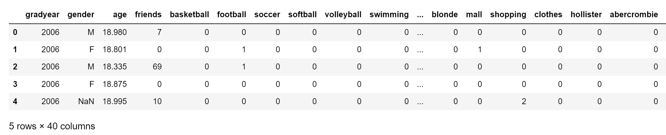
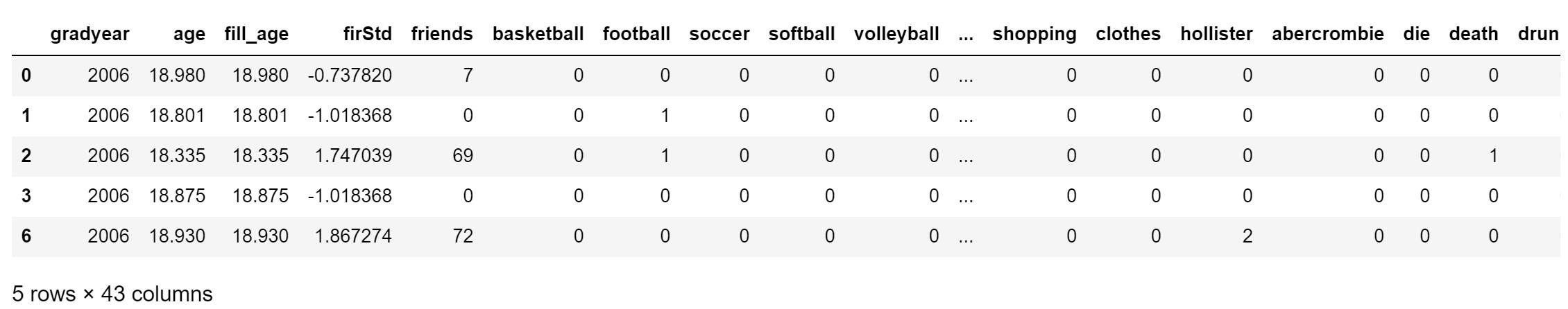
(1)读取数据并查看数据的前5行;
(2)查看数据集整体情况;
(3)查看缺失值的统计性描述分布情况;
(4)假设青少年的年龄范围为13-20岁,我们将不在此范围的数据记为缺失值,重新统计缺失值数目;
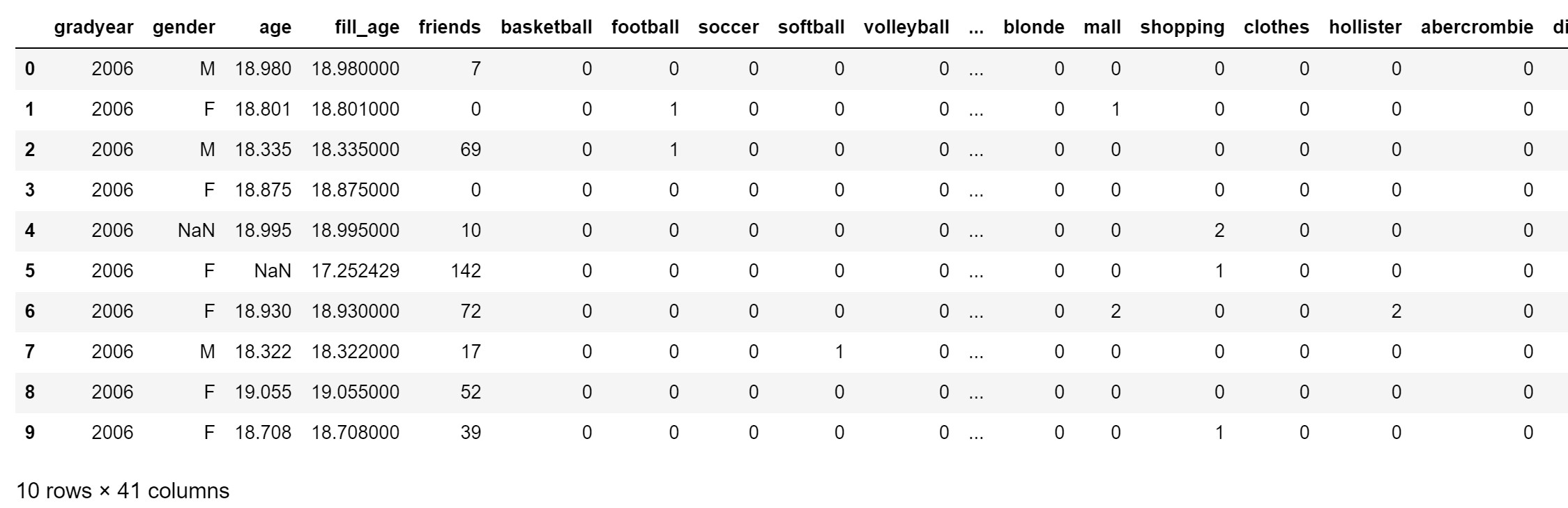
(5)选取年龄的均值填充年龄缺失值;
(6)统计性别缺失值并将其删除;
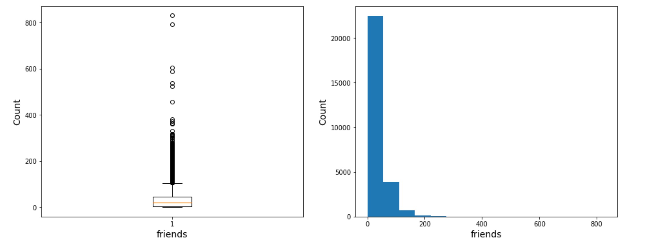
(7)采用箱线图对friend列数据进行异常值检测;
(8)删除异常值(规定:超过上四分位+1.5倍IQR距离,或者下四分位-1.5倍IQR距离的点为异常值,四分位距(IQR)就是上四分位与下四分位的差值,我们以IQR的1.5倍为标准)
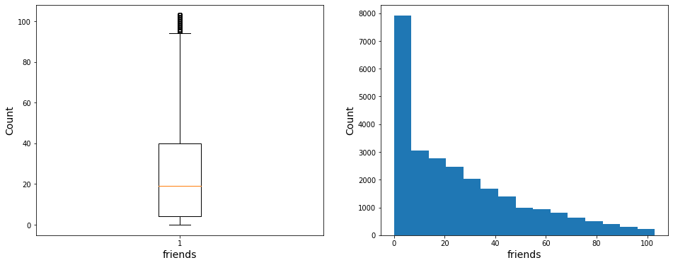
(9)采用箱线图查看异常值剔除后的数据分布情况;
(10)对friend列进行标准差标准化处理;
(11)对gender列进行One-Hot编码;
(12)采用等距离散化方法对friends进行划分。
三、题解
1
2
3
4
5
6
|
import pandas as pd
df = pd.read_csv('teenager_sns.csv', sep = ',')
df.head(5)
|
1
2
3
4
5
6
7
8
9
10
11
12
13
14
15
16
17
18
19
20
21
22
23
24
25
26
27
28
29
30
31
32
33
34
35
36
37
38
39
40
41
42
43
44
45
46
47
| <class 'pandas.core.frame.DataFrame'>
RangeIndex: 30000 entries, 0 to 29999
Data columns (total 40 columns):
# Column Non-Null Count Dtype
--- ------ -------------- -----
0 gradyear 30000 non-null int64
1 gender 27276 non-null object
2 age 24914 non-null float64
3 friends 30000 non-null int64
4 basketball 30000 non-null int64
5 football 30000 non-null int64
6 soccer 30000 non-null int64
7 softball 30000 non-null int64
8 volleyball 30000 non-null int64
9 swimming 30000 non-null int64
10 cheerleading 30000 non-null int64
11 baseball 30000 non-null int64
12 tennis 30000 non-null int64
13 sports 30000 non-null int64
14 cute 30000 non-null int64
15 sex 30000 non-null int64
16 sexy 30000 non-null int64
17 hot 30000 non-null int64
18 kissed 30000 non-null int64
19 dance 30000 non-null int64
20 band 30000 non-null int64
21 marching 30000 non-null int64
22 music 30000 non-null int64
23 rock 30000 non-null int64
24 god 30000 non-null int64
25 church 30000 non-null int64
26 jesus 30000 non-null int64
27 bible 30000 non-null int64
28 hair 30000 non-null int64
29 dress 30000 non-null int64
30 blonde 30000 non-null int64
31 mall 30000 non-null int64
32 shopping 30000 non-null int64
33 clothes 30000 non-null int64
34 hollister 30000 non-null int64
35 abercrombie 30000 non-null int64
36 die 30000 non-null int64
37 death 30000 non-null int64
38 drunk 30000 non-null int64
39 drugs 30000 non-null int64
dtypes: float64(1), int64(38), object(1)
memory usage: 9.2+ MB
|
1
2
3
|
df['gender'].describe()
|
1
2
3
4
5
| count 27276
unique 2
top F
freq 22054
Name: gender, dtype: object
|
1
2
3
4
5
6
7
8
9
| count 24914.000000
mean 17.993949
std 7.858054
min 3.086000
25% 16.312000
50% 17.287000
75% 18.259000
max 106.927000
Name: age, dtype: float64
|
1
2
3
|
df['age'].isnull().sum()
|
1
2
3
4
5
|
import numpy as np
df['age'] = df.apply(lambda x : np.nan if (x['age']<13.0) | (x['age']>20.0) else x['age'], axis = 1)
df['age'].isnull().sum()
|
1
2
3
4
5
|
df.insert(3, 'fill_age', df['age'].fillna(df['age'].mean()))
df.head(10)
|
1
2
3
4
|
df['gender'].isnull().sum()
df.dropna(subset=['gender'], inplace=True)
|
1
| df['gender'].isnull().sum()
|
1
2
3
4
5
6
7
8
9
10
11
12
13
14
15
16
17
|
import matplotlib.pyplot as plt
fig = plt.figure(figsize=(16,6))
plt.subplot(1, 2, 1)
plt.boxplot(x = df.friends)
plt.xlabel('friends', fontsize = 14)
plt.ylabel('Count', fontsize = 14)
plt.subplot(1, 2, 2)
plt.hist(df.friends, bins = 15)
plt.xlabel('friends', fontsize = 14)
plt.ylabel('Count', fontsize = 14)
plt.show()
|
1
2
3
4
5
6
7
8
9
10
|
IQR = df['friends'].quantile(0.75) - df['friends'].quantile(0.25)
up = df['friends'].quantile(0.75) + IQR*1.5
down = df['friends'].quantile(0.25) - IQR*1.5
teenager = df[ (df['friends'] > down) & (df['friends'] < up)]
teenager['friends'].describe()
|
1
2
3
4
5
6
7
8
9
| count 26122.000000
mean 25.409425
std 24.951122
min 0.000000
25% 4.000000
50% 19.000000
75% 40.000000
max 103.000000
Name: friends, dtype: float64
|
1
2
3
4
5
6
7
8
9
10
11
12
13
14
15
16
17
|
import matplotlib.pyplot as plt
fig = plt.figure(figsize=(16,6))
plt.subplot(1, 2, 1)
plt.boxplot(x = teenager.friends)
plt.xlabel('friends', fontsize = 14)
plt.ylabel('Count', fontsize = 14)
plt.subplot(1, 2, 2)
plt.hist(teenager.friends, bins = 15)
plt.xlabel('friends', fontsize = 14)
plt.ylabel('Count', fontsize = 14)
plt.show()
|
1
2
3
4
5
6
7
8
9
|
def StandarScaler(data):
data=(data - data.mean()) / data.std()
return data
teenager.insert(4, 'firStd', StandarScaler(teenager['friends']))
teenager.head()
|

1
2
3
4
|
pd.get_dummies(teenager).head()
|
1
2
3
4
5
6
|
col_new = 'group'
teenager.insert(4, col_new, pd.cut(teenager['friends'], 3, labels = ['好友少', '好友正常', '好友多']))
teenager.head()
|

1
| teenager['group'].value_counts()
|
1
2
3
4
| 好友少 18226
好友正常 5847
好友多 2049
Name: group, dtype: int64
|
四、参考资料
teenager 数据集下载